How to process Umbrella Sampling in GROMACS
Umbrella Sampling (US)
Introduction
Generally, the whole process of computational US simulation can be divided into seven steps:
 – Generate topology
 – Define unit cell
 – Solvate and add ions
 – Minimization and equilibration
 – Generate configuration
 – Umbrella sampling
 – Data analysis
The files that we need to proceed simulation:
 –input.pdb
 –parameter files (for each step if it need)
 –Force field
Procedures
Step 1
Code:
pdb2gmx -f input.pdb -ignh -ter -o output.gro
Force field:
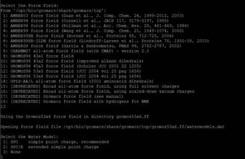
Choose the force field you need in list below:
Tips:
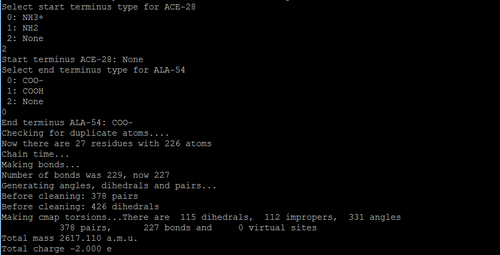
In this step, after you chose the force field, you need to select the type of ions for each terminal of each chain.
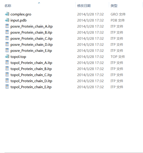
Then, you will see some new files generated in your specified directory.
Step 2
Code:
editconf -f output.gro -o boxed.gro -center x y z -box X Y Z
Here the x, y and z are used to define the position of the mass center in the box, and the X, Y and Z are used to define the size of the box. The unit is nm.
GROMACS calculates distances while simultaneously taking periodicity into account. This, if you have a 10-nm box, and you pull over a distance greater than 5.0 nm, the periodic distance becomes the reference distance for the pulling, and this distance is actually less than 5.0 nm! This fact will significantly affect results, since the distance you think you are pulling is not what is actually calculated.
Tips:
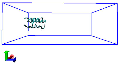
You can visualize the location of the protofibril within the box using, for example, VMD. Load the structure in VMD and open the Tk console. Type the following (note that > indicates the Tk prompt, not something you actually type):
pbc box
You should see something like the following in the VMD window:
Step 3
Code:
genbox -cp boxed.gro -cs spc216.gro -o solv.gro -p topol.top
grompp -f ions.mdp -c solv.gro -p topol.top -o ions.tpr
genion -s ions.tpr -o solv_ions.gro -p topol.top -pname NA -nname CL -neutral -conc 0.1
Parameter file:
The contents of the parameter file are showed in below:
; ions.mdp - used as input into grompp to generate ions.tpr
; Parameters describing what to do, when to stop and what to save
integrator  = steep     ; Algorithm (steep = steepest descent minimization)
emtol       = 1000.0    ; Stop minimization when the maximum force < 1000.0 kJ/mol/nm
emstep      = 0.01      ; Energy step size
nsteps      = 50000     ; Maximum number of (minimization) steps to perform

; Parameters describing how to find the neighbors of each atom and how to calculate the interactions
nstlist     = 1         ; Frequency to update the neighbor list and long range forces
ns_type     = grid      ; Method to determine neighbor list (simple, grid)
rlist       = 1.4       ; Cut-off for making neighbor list (short range forces)
coulombtype = PME       ; Treatment of long range electrostatic interactions
rcoulomb    = 1.4       ; Short-range electrostatic cut-off
rvdw        = 1.4       ; Short-range Van der Waals cut-off
pbc         = xyz       ; Periodic Boundary Conditions
Tips:
Step 4
Code:
grompp -f minim.mdp -c solv_ions.gro -p topol.top -o em.tpr
mdrun -v -deffnm em
grompp -f npt.mdp -c em.gro -p topol.top -o npt.tpr
mdrun -deffnm npt
Parameter file:
; minimi.mdp - error
title       = NPT Equilibration
define      = -DPOSRES          ; position restrain the protein
; Run parameters
integrator  = md                ; leap-frog integrator
nsteps      = 50000             ; 2 * 50000 = 100 ps
dt          = 0.002             ; 2 fs
; Output control
nstxout     = 1000              ; save coordinates every 2 ps
nstvout     = 1000              ; save velocities every 2 ps
nstenergy   = 1000              ; save energies every 2 ps
nstlog      = 1000              ; update log file every 2 ps
; Bond parameters
continuation         = no        ; Initial simulation
constraint_algorithm = lincs     ; holonomic constraints
constraints          = all-bonds ; all bonds (even heavy atom-H bonds) constrained
lincs_iter           = 1         ; accuracy of LINCS
lincs_order          = 4         ; also related to accuracy
; Neighborsearching
ns_type     = grid              ; search neighboring grid cels
nstlist     = 5                 ; 10 fs
rlist       = 1.4               ; short-range neighborlist cutoff (in nm)
rcoulomb    = 1.4               ; short-range electrostatic cutoff (in nm)
rvdw        = 1.4               ; short-range van der Waals cutoff (in nm)
; Electrostatics
coulombtype     = PME           ; Particle Mesh Ewald for long-range electrostatics
pme_order       = 4             ; cubic interpolation
fourierspacing  = 0.16          ; grid spacing for FFT
; Temperature coupling is on
tcoupl      = Berendsen             ; Weak coupling for initial equilibration
tc-grps     = Protein   Non-Protein ; two coupling groups - more accurate
tau_t       = 0.1       0.1         ; time constant, in ps
ref_t       = 310       310         ; reference temperature, one for each group, in K
; Pressure coupling is on
pcoupl              = Berendsen     ; Pressure coupling on in NPT, also weak coupling
pcoupltype          = isotropic     ; uniform scaling of x-y-z box vectors
tau_p               = 2.0           ; time constant, in ps
ref_p               = 1.0           ; reference pressure (in bar)
compressibility     = 4.5e-5        ; isothermal compressibility, bar^-1
refcoord_scaling    = com
; Periodic boundary conditions
pbc     = xyz                   ; 3-D PBC
; Dispersion correction
DispCorr    = EnerPres          ; account for cut-off vdW scheme
; Velocity generation
gen_vel     = yes               ; Velocity generation is on
gen_temp    = 310               ; temperature for velocity generation
gen_seed    = -1                ; random seed
; COM motion removal
; These options remove COM motion of the system
nstcomm         = 10
comm-mode       = Linear
comm-grps       = System
Tips:
Step 5
Code:
Parameter file:
Tips:
Step 6
Code:
Parameter file:
Tips:
Step 7
Code:
Parameter file:
Tips:
Basis of sampling techniques
What is Free Energy
The thermodynamic free energy is the amount of work that a thermodynamic system can perform. The concept is useful in the thermodynamics of chemical or thermal processes in engineering and science. The free energy is the internal energy of a system minus the amount of energy that cannot be used to perform work. This unusable energy is given by the entropy of a system multiplied by the temperature of the system.
Like the internal energy, the free energy is a thermodynamic state function. Energy is a generalization of free energy.
Generally, it can be classified into different types, such as the commonest ones:
Helmholtz free energy
The energy that can be converted into work at a constant temperature and volume. It can be used to calculate the total potential energy of the system.
Gibbs free energy
The energy that can be converted into work at a uniform temperature and pressure throughout a system. The Gibbs free energy is the measure of the system to do useful work, which is measurement of spontaneous system process.
Calculation of Free Energy
Generally, there are several methods for calculating free energy, for instance, the free energy perturbation method (FEP), the thermodynamic integration method (TI), umbrella sampling (US), the adaptive bias force method (ABF) and so forth. The adaptive bias force method is the improvement of the umbrella sampling, and it is commonly used as US.
The free energy perturbation method (FEP):
The thermodynamic integration method (TI):
Umbrella sampling (US):
The adaptive bias force method (ABF):
Theoretical process of Umbrella Sampling
Computational process
Main References
1. File:Free energy calculations theory and applications in chemistry and biology.pdf


